Speeding up MD simulations in explicit solvent.

Given my earlier blog entry, it turns out that implicit solvent simulations are out of the questions. Gromacs simulations do not scale well due to the lack of support for parallel Generalised Born Implicit Solvent (GBIS) and I am still of the opinion that explicit protein-water-protein interactions are fundamental for an accurate protein fold. I am very confident that most published explicit solvent simulations that do not try and break the nanosecond to microsecond barrier use a time step of 0.002 ps (2 fs) along with LINCS order and iteration as per default (4 and 1, respectively). Until now, I’ve never tried to move into the microsecond scale and therefore, tweaking the time step and LINCS parameters have never been a priority.

Speeding up by increasing the time step (dt)
As per the Gromacs documentation and the original publication “P-LINCS: A Parallel Linear Constraint Solver for Molecular Simulations”, the LINCS order (lincs_order) must be set to 6 for larger time steps. The LINCS iteration can be left unless dealing with an NVE ensemble in which case it is recommended to set the iteration to 2. The original publication demonstrates energy conservation at a time step of 0.005 ps with a LINCS order and iteration of 6 and 1, respectively. Although there is a very slight computational overhead with an increased LINCS order, an increase in the time step will save on significant computational time.

The steps to run simulations using a dt of 0.005 are:

1. During execution of pdb2gmx specify -vsite hydrogens -heavyh 
2. For the LINCS constraints during the energy minimisation step constraints = none It will be very hard to avoid LINCS warnings during the minimisation step otherwise. Use SETTLE for a rigid water model (this should be on by default).
3. Maintain the rigid water model, switch constraints = all-bonds, lincs_iter = 1 and lincs_order = 6. 
4. I took to performing a 400 ps NVT followed by a 400 ps NPT simulation using a dt of 0.002, whilst maintaining position restraints on the protein.
5. Restraints were removed, the pressure coupling was switched to Parrinello-Rahman and the system was allowed to continue equilibrating for a further 400 ps with a dt of 0.002.
6. The time step was incremented to 0.003, 0.004 and 0.005 over a series of 400 ps NPT simulations.

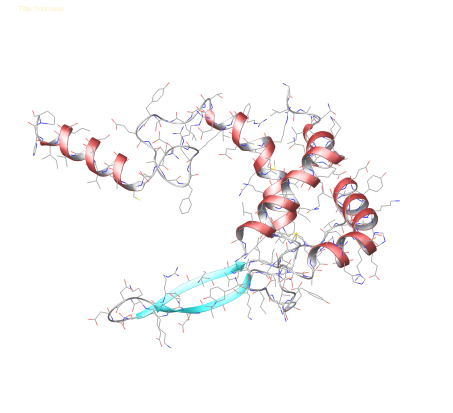
Following these steps and applying the required mdp settings, simulations of the structure visible below in a TIP3P water solvent over 1 node with 4 cores (Intel i5 2.60 GHz processor) yields:

• 1.269 ns/day at dt of 2 fs
• 2.587 ns/day at dt of 4 fs

Moving this simulation over to a node capable of executing 16 MPI threads I expect approximately 21.985 ns/day. Alternatively, buy a good GPU. But, given that I planned to run simulations on my own personal 32 core machine at home, I have what I’ve got.